A visual course · side project · 2026

Balancing on a ball.

I am building a ballbot: a robot that stands on a single sphere and drives it with three omni-wheels. Before any hardware, the model. Derive the kinematics, the full non-linear dynamics and the linear model a controller needs — then try to keep it upright yourself.

3omni-wheels, 120° apart
6independent speeds
+5.58rad/s unstable pole
Scroll to begin · drag the scene to rotate
Chapter 1 · The robot

One ball, one body, three wheels.

Everything starts from a sketch: name every body, parameter and coordinate before writing a single equation.

Bodies

A body A balances on a ball B that rolls on the floor 0. Three omni-wheels W₁, W₂, W₃, mounted on the body, touch the ball at a zenith angle α\alpha and drive it. Their passive rollers let the ball slide along each wheel's axle, so every wheel only pushes along its own rolling direction.

0Floor, inertial frame, world axes ex,ey,ez\mathbf e_x,\mathbf e_y,\mathbf e_z (z up)
BBall, solid sphere, IB=25mBR2I_B=\tfrac25 m_B R^2
ABody: drive plate, motors, battery, mast, computer, IMU, lidar. Centre of mass G.
W₁₋₃Omni-wheels, massless in the model; motor torque τi\tau_i between A and Wᵢ
H, TTwo massless virtual bodies that carry the coordinates: heading and tilt

Parameters

Side view. G sits at height ll above the ball centre; each wheel touches the ball at α\alpha from the vertical.

RRball radius120 mm
rwr_womni-wheel radius50 mm
α\alphazenith angle of the contacts50°
γi\gamma_iwheel azimuths0°, 120°, 240°
llheight of G above the ball centre300 mm
mB, IBm_B,\ I_Bball mass, inertia2.4 kg, 25mBR22.4\ \text{kg},\ \tfrac25 m_BR^2
mAm_Abody mass12 kg
IA, IAzI_A,\ I_{Az}tilt and yaw inertia about G0.9, 0.12 kg·m²

Coordinates

The ball centre is at c=(xB, yB, R)\mathbf c=(x_B,\,y_B,\,R). The body orientation is described by three angles: heading ψ\psi, pitch ϑ\vartheta and roll φ\varphi. The ball has its own orientation, and each wheel its angle θi\theta_i.

Top view: heading frame rotated by psi and the three omni-wheels
Top view. The heading frame H is the floor frame turned by ψ\psi; wheels sit at azimuths γi=γ0+(i−1) 120∘\gamma_i=\gamma_0+(i-1)\,120^\circ.
Degrees of freedom
11 coordinates, 5 rolling constraints (2 floor + 3 wheels): 6 independent speeds x˙B,y˙B,ψ˙,ϑ˙,φ˙,ωz\dot x_B,\dot y_B,\dot\psi,\dot\vartheta,\dot\varphi,\omega_z. Three motors for six speeds: the ballbot is underactuated — which is exactly why it has to balance.
Chapter 2 · Parametrization

Yaw, pitch, roll.

Three successive rotations, one per joint of the chain floor → H → T → A. A formalism that is easy to get wrong, so let's play with it.

Three elementary rotations

A rotation matrix stores the new axes, written in the old ones, as its columns. With the right-hand rule, the three elementary rotations are
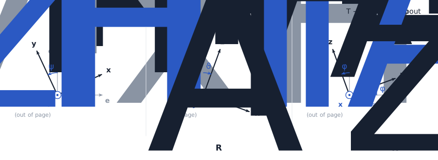
Rx(a)=(1000cos⁡a−sin⁡a0sin⁡acos⁡a),Ry(a)=(cos⁡a0sin⁡a010−sin⁡a0cos⁡a)\mathbf R_x(a)=\begin{pmatrix}1&0&0\\0&\cos a&-\sin a\\0&\sin a&\cos a\end{pmatrix},\qquad \mathbf R_y(a)=\begin{pmatrix}\cos a&0&\sin a\\0&1&0\\-\sin a&0&\cos a\end{pmatrix}
Rz(a)=(cos⁡a−sin⁡a0sin⁡acos⁡a0001)\mathbf R_z(a)=\begin{pmatrix}\cos a&-\sin a&0\\\sin a&\cos a&0\\0&0&1\end{pmatrix}
Rotation chain 0 to H to T to A: yaw psi, pitch vartheta, roll varphi
Thin grey: old axes; bold: new axes; the rotation axis points out of the page.

The minus sign of Ry\mathbf R_y sits bottom-left: for a rotation about y the cyclic order is z → x. On the right, the robot plays the chain: yaw ψ\psi about ez\mathbf e_z gives H, pitch ϑ\vartheta about yH\mathbf y_H gives T, roll φ\varphi about xT\mathbf x_T gives A.

Compose them yourself

RA=Rz(ψ) Ry(ϑ) Rx(φ)\mathbf R_A=\mathbf R_z(\psi)\,\mathbf R_y(\vartheta)\,\mathbf R_x(\varphi)

Read left to right: rotate about z, then about the new y, then about the newest x (intrinsic, how the joints are stacked). Read right to left: the same rotations about the fixed axes, in reverse order. Each ring on the right is one joint.

gimbal lock at ϑ = ±90° · det = cos ϑ = 0.940
RA=(0.814−0.5600.1570.4700.7920.389−0.342−0.2430.908)\mathbf R_A = \begin{pmatrix} 0.814 & -0.560 & 0.157 \\ 0.470 & 0.792 & 0.389 \\ -0.342 & -0.243 & 0.908 \end{pmatrix}
Third column = body axis zA\mathbf z_A, the direction from the ball centre to G.

Angle rates are not the angular velocity

Angular velocities add along the chain, each joint turning about its own axis:

ωA=ψ˙ zH+ϑ˙ yT+φ˙ xA\boldsymbol\omega_A=\dot\psi\,\mathbf z_H+\dot\vartheta\,\mathbf y_T+\dot\varphi\,\mathbf x_A

Bringing every axis into body components gives

Body angular velocity
ωA(A)=(φ˙−ψ˙sin⁡ϑϑ˙cos⁡φ+ψ˙cos⁡ϑsin⁡φψ˙cos⁡ϑcos⁡φ−ϑ˙sin⁡φ)\boldsymbol\omega_A^{(A)}=\begin{pmatrix}\dot\varphi-\dot\psi\sin\vartheta\\ \dot\vartheta\cos\varphi+\dot\psi\cos\vartheta\sin\varphi\\ \dot\psi\cos\vartheta\cos\varphi-\dot\vartheta\sin\varphi\end{pmatrix}

The map from (φ˙,ϑ˙,ψ˙)(\dot\varphi,\dot\vartheta,\dot\psi) to ωA\boldsymbol\omega_A has determinant cos⁡ϑ\cos\vartheta: at ϑ=±90∘\vartheta=\pm90^\circ yaw and roll line up (gimbal lock). A balancing ballbot never gets there. Drawn on the right for ψ˙,ϑ˙,φ˙=0.5, 0.35, −0.25\dot\psi,\dot\vartheta,\dot\varphi=0.5,\,0.35,\,-0.25 rad/s at the angles you set.

Chapter 3 · Kinematics

Rolling, without slipping.

Two kinds of contact: ball on floor, wheel on ball. Each is a constraint on velocities, not on positions.

Ball on the floor

The ball particle touching the floor, at c−R ez\mathbf c-R\,\mathbf e_z, has zero velocity:

c˙+ωB×(−R ez)=0⟹x˙B=R ωB,y,y˙B=−R ωB,x\dot{\mathbf c}+\boldsymbol\omega_B\times(-R\,\mathbf e_z)=\mathbf 0\quad\Longrightarrow\quad \dot x_B=R\,\omega_{B,y},\qquad \dot y_B=-R\,\omega_{B,x}

The vertical row reads 0 = 0: the floor does not fix the spin ωB,z\omega_{B,z}. Only the wheels can spin the ball about the vertical.

Three vectors per wheel

In body axes, wheel ii touches the ball at R niR\,\mathbf n_i, turns about its axle ai\mathbf a_i, and its rim rolls along ti\mathbf t_i:

ni=(sin⁡αcos⁡γisin⁡αsin⁡γicos⁡α),  ai=(cos⁡αcos⁡γicos⁡αsin⁡γi−sin⁡α)\mathbf n_i=\begin{pmatrix}\sin\alpha\cos\gamma_i\\\sin\alpha\sin\gamma_i\\\cos\alpha\end{pmatrix},\ \ \mathbf a_i=\begin{pmatrix}\cos\alpha\cos\gamma_i\\\cos\alpha\sin\gamma_i\\-\sin\alpha\end{pmatrix}
ti=ni×ai=(−sin⁡γicos⁡γi0)\mathbf t_i=\mathbf n_i\times\mathbf a_i=\begin{pmatrix}-\sin\gamma_i\\\cos\gamma_i\\0\end{pmatrix}
Meridian-plane detail of omni-wheel i on the ball
Wheel ii in its meridian plane (the plane of zA\mathbf z_A and ni\mathbf n_i). ti\mathbf t_i points into the page (⊗).

In 3D: black ni\mathbf n_i, grey ai\mathbf a_i, blue ti\mathbf t_i. The rollers make the ball free to slide along ai\mathbf a_i; only motion along ti\mathbf t_i is constrained.

The wheel equation

Rim and ball surface must agree along the rolling direction. Both bodies share the ball centre, so only rotations matter:

Omni-wheel constraint
rw θ˙i=R (ωA−ωB)⋅air_w\,\dot\theta_i=R\,(\boldsymbol\omega_A-\boldsymbol\omega_B)\cdot\mathbf a_i

Stacked for the three wheels (rows of J\mathbf J are aiT\mathbf a_i^{\mathsf T}, here γ0=0\gamma_0=0):

θ˙=RrwJ(ωA−ωB)(A),J=(cos⁡α0−sin⁡α−12cos⁡α32cos⁡α−sin⁡α−12cos⁡α−32cos⁡α−sin⁡α)\dot{\boldsymbol\theta}=\frac{R}{r_w}\mathbf J(\boldsymbol\omega_A-\boldsymbol\omega_B)^{(A)},\quad \mathbf J=\begin{pmatrix}\cos\alpha&0&-\sin\alpha\\-\tfrac12\cos\alpha&\tfrac{\sqrt3}2\cos\alpha&-\sin\alpha\\-\tfrac12\cos\alpha&-\tfrac{\sqrt3}2\cos\alpha&-\sin\alpha\end{pmatrix}

J\mathbf J is invertible for 0<α<π/20<\alpha<\pi/2: any relative rotation between ball and body is reachable with three wheels. On the right, the wheels turn at exactly this rate while the ball rolls.

Inverse of JJ⁻¹
J−1=(23cos⁡α−13cos⁡α−13cos⁡α013cos⁡α−13cos⁡α−13sin⁡α−13sin⁡α−13sin⁡α)\mathbf J^{-1}=\begin{pmatrix}\tfrac{2}{3\cos\alpha}&-\tfrac{1}{3\cos\alpha}&-\tfrac{1}{3\cos\alpha}\\0&\tfrac{1}{\sqrt3\cos\alpha}&-\tfrac{1}{\sqrt3\cos\alpha}\\-\tfrac{1}{3\sin\alpha}&-\tfrac{1}{3\sin\alpha}&-\tfrac{1}{3\sin\alpha}\end{pmatrix}
Chapter 4 · Newton–Euler

Six equations, three motors.

The full non-linear 3D dynamics, written for the body and the ball separately, then glued together by the motor torques.

Free-body diagram

Rigid bodies, massless wheels and ideal rollers, rolling without slip. Because the wheels are massless, each motor torque passes straight through as a couple between body and ball. Power balance ∑iτiθ˙i=T⋅(ωA−ωB)\sum_i\tau_i\dot\theta_i=\mathbf T\cdot(\boldsymbol\omega_A-\boldsymbol\omega_B) gives

T=Rrw∑i=13τi aion the body,−T on the ball\mathbf T=\frac{R}{r_w}\sum_{i=1}^{3}\tau_i\,\mathbf a_i\quad\text{on the body},\qquad -\mathbf T\ \text{on the ball}

On the right, the body is lifted off the ball. F\mathbf F: contact force of ball on body, F0\mathbf F_0: floor reaction, ρ=BG→=l zA\boldsymbol\rho=\overrightarrow{BG}=l\,\mathbf z_A.

Newton–Euler, then eliminate the contact forces

body:mA aG=F−mAg ezIAω˙A+ωA×IAωA=T−ρ×Fball:mB c¨=F0−F−mBg ezIB ω˙B=−T−R ez×F0\begin{aligned}\text{body:}\quad& m_A\,\mathbf a_G=\mathbf F-m_Ag\,\mathbf e_z\\ & \mathbf I_A\dot{\boldsymbol\omega}_A+\boldsymbol\omega_A\times\mathbf I_A\boldsymbol\omega_A=\mathbf T-\boldsymbol\rho\times\mathbf F\\[4pt] \text{ball:}\quad& m_B\,\ddot{\mathbf c}=\mathbf F_0-\mathbf F-m_Bg\,\mathbf e_z\\ & I_B\,\dot{\boldsymbol\omega}_B=-\mathbf T-R\,\mathbf e_z\times\mathbf F_0\end{aligned}

Substituting F\mathbf F and F0\mathbf F_0 leaves six equations in the angular accelerations and the motor torques:

Equations of motion (full, non-linear)
IAω˙A+ωA×IAωA+mA ρ×(aG+g ez)=Rrw∑iτi aiIB ω˙B+R ez×(mB c¨+mA aG)=−Rrw∑iτi ai\begin{aligned} &\mathbf I_A\dot{\boldsymbol\omega}_A+\boldsymbol\omega_A\times\mathbf I_A\boldsymbol\omega_A+m_A\,\boldsymbol\rho\times(\mathbf a_G+g\,\mathbf e_z)\\&\qquad=\frac{R}{r_w}\sum_i\tau_i\,\mathbf a_i\\[6pt] &I_B\,\dot{\boldsymbol\omega}_B+R\,\mathbf e_z\times\big(m_B\,\ddot{\mathbf c}+m_A\,\mathbf a_G\big)\\&\qquad=-\frac{R}{r_w}\sum_i\tau_i\,\mathbf a_i\end{aligned}
Every term, expandednon-linear

All vectors in world axes. Orientation and centre of mass:

zA=(cos⁡ψsin⁡ϑcos⁡φ+sin⁡ψsin⁡φsin⁡ψsin⁡ϑcos⁡φ−cos⁡ψsin⁡φcos⁡ϑcos⁡φ),ρ=l zA\mathbf z_A=\begin{pmatrix}\cos\psi\sin\vartheta\cos\varphi+\sin\psi\sin\varphi\\\sin\psi\sin\vartheta\cos\varphi-\cos\psi\sin\varphi\\\cos\vartheta\cos\varphi\end{pmatrix},\qquad \boldsymbol\rho=l\,\mathbf z_A

Accelerations (rigid body, then rolling):

aG=c¨+ω˙A×ρ+ωA×(ωA×ρ),c¨=(x¨B,y¨B,0)=−R ez×ω˙B\mathbf a_G=\ddot{\mathbf c}+\dot{\boldsymbol\omega}_A\times\boldsymbol\rho+\boldsymbol\omega_A\times(\boldsymbol\omega_A\times\boldsymbol\rho),\qquad \ddot{\mathbf c}=(\ddot x_B,\ddot y_B,0)=-R\,\mathbf e_z\times\dot{\boldsymbol\omega}_B

World inertia of the axisymmetric body, which changes as it tilts (hence the gyroscopic term):

IA=RA diag(IA,IA,IAz) RAT=IA 1+(IAz−IA) zAzAT\mathbf I_A=\mathbf R_A\,\mathrm{diag}(I_A,I_A,I_{Az})\,\mathbf R_A^{\mathsf T}=I_A\,\mathbf 1+(I_{Az}-I_A)\,\mathbf z_A\mathbf z_A^{\mathsf T}

Angular velocities, from chapter 2 and the ball speeds ω=(ωx,ωy,ωz)\boldsymbol\omega=(\omega_x,\omega_y,\omega_z) given in H axes:

ωA=RA ωA(A),ωB=ψ˙ ez+Rz(ψ) ω\boldsymbol\omega_A=\mathbf R_A\,\boldsymbol\omega_A^{(A)},\qquad \boldsymbol\omega_B=\dot\psi\,\mathbf e_z+\mathbf R_z(\psi)\,\boldsymbol\omega

Cross-checked numerically (9–10 digits) against the equations KineSketch generates symbolically from the same sketch (sympy, Kane's method).

Why it has to balance

Add the two equations: the motors cancel. What is left is the angular-momentum balance about the floor contact point:

Balance equations — no motor acts on them
IAω˙A+ωA×IAωA+mA ρ×(aG+g ez)+IBω˙B+R ez×(mBc¨+mAaG)=0\begin{aligned}&\mathbf I_A\dot{\boldsymbol\omega}_A+\boldsymbol\omega_A\times\mathbf I_A\boldsymbol\omega_A+m_A\,\boldsymbol\rho\times(\mathbf a_G+g\,\mathbf e_z)\\&\quad+I_B\dot{\boldsymbol\omega}_B+R\,\mathbf e_z\times(m_B\ddot{\mathbf c}+m_A\mathbf a_G)=\mathbf 0\end{aligned}

Gravity on the tilted body, mA ρ×g ezm_A\,\boldsymbol\rho\times g\,\mathbf e_z, can only be countered by accelerating the ball and the body. The motors never push on the world directly: they move the ball under the body. Only the ball spin about the vertical is driven directly, by the vertical row of the ball equation: IBω˙B,z=−TzI_B\dot\omega_{B,z}=-T_z.

Chapter 5 · Planar model

Lean to accelerate.

Cut the problem along one axis: motion along x, pitch ϑ. Two degrees of freedom, still fully non-linear.

The sagittal plane

With ψ=φ=0\psi=\varphi=0, rolling ωB,y=x˙B/R\omega_{B,y}=\dot x_B/R, and τ=−Ty\tau=-T_y the equivalent pitch torque:

Side view of the ballbot in the x–z plane, body pitched by vartheta
Side view, ey\mathbf e_y into the page.
Planar equations of motion
(mB+IBR2+mAmAlcos⁡ϑmAlcos⁡ϑIA+mAl2)(x¨Bϑ¨)+(−mAlsin⁡ϑ ϑ˙2−mAglsin⁡ϑ)=(1/R−1)τ\begin{aligned}&\begin{pmatrix}m_B+\frac{I_B}{R^2}+m_A& m_Al\cos\vartheta\\ m_Al\cos\vartheta& I_A+m_Al^2\end{pmatrix}\begin{pmatrix}\ddot x_B\\\ddot\vartheta\end{pmatrix}\\&\qquad+\begin{pmatrix}-m_Al\sin\vartheta\,\dot\vartheta^2\\-m_Agl\sin\vartheta\end{pmatrix}=\begin{pmatrix}1/R\\-1\end{pmatrix}\tau\end{aligned}

With γ0=0\gamma_0=0, τ=Rrw32cos⁡α (τ3−τ2)\tau=\tfrac{R}{r_w}\tfrac{\sqrt3}{2}\cos\alpha\,(\tau_3-\tau_2): wheels 2 and 3 push, wheel 1 only rolls along. A positive torque accelerates the ball forward and pushes the body backwards — the −1-1 in the right-hand side.

The forward lean

For a steady acceleration aa (ϑ¨=ϑ˙=0\ddot\vartheta=\dot\vartheta=0), gravity must supply the opposite moment, so the body leans forward:

mAglsin⁡ϑ=mAl acos⁡ϑ+R(mB+IBR2+mA)am_Agl\sin\vartheta=m_Al\,a\cos\vartheta+R\Big(m_B+\frac{I_B}{R^2}+m_A\Big)a

The last term is the drive reaction. It makes the lean larger than the naive pendulum answer tan⁡ϑ=a/g\tan\vartheta=a/g.

lean from the model8.80°
naive atan(a/g)5.82°
ratio1.51×
The ball oscillates with acceleration amplitude a_max; the body tracks the steady lean of the formula at every instant.
Chapter 6 · Linearization

One unstable pole.

A controller is designed on a linear model. Linearize about the upright equilibrium.

Small angles

About ϑ=0\vartheta=0: sin⁡ϑ≈ϑ\sin\vartheta\approx\vartheta, cos⁡ϑ≈1\cos\vartheta\approx1, and ϑ˙2\dot\vartheta^2 is second order. The planar model becomes

Linearized about upright
(mB+IB/R2+mAmAlmAlIA+mAl2)⏟M(x¨Bϑ¨)−(0mAgl ϑ)=(1/R−1)τ\begin{aligned}&\underbrace{\begin{pmatrix}m_B+I_B/R^2+m_A& m_Al\\ m_Al& I_A+m_Al^2\end{pmatrix}}_{\mathbf M}\begin{pmatrix}\ddot x_B\\\ddot\vartheta\end{pmatrix}\\&\qquad-\begin{pmatrix}0\\m_Agl\,\vartheta\end{pmatrix}=\begin{pmatrix}1/R\\-1\end{pmatrix}\tau\end{aligned}

On the right: the non-linear model with the motors off, released from 1°. It falls in well under a second.

State space

With the state s=(xB,ϑ,x˙B,ϑ˙)\mathbf s=(x_B,\vartheta,\dot x_B,\dot\vartheta) and s˙=As+Bτ\dot{\mathbf s}=\mathbf A\mathbf s+\mathbf B\tau, invert M\mathbf M (det = 17.45 kg²m²):

A=(001000010− mAgl M12/det⁡M000mAgl M11/det⁡M00)\mathbf A=\begin{pmatrix}0&0&1&0\\0&0&0&1\\0&-\,m_Agl\,M_{12}/\det\mathbf M&0&0\\0&m_Agl\,M_{11}/\det\mathbf M&0&0\end{pmatrix}
A=(001000010−7.28500031.08100),B=(001.152−2.599)\mathbf A=\begin{pmatrix}0&0&1&0\\0&0&0&1\\0&-7.285&0&0\\0&31.081&0&0\end{pmatrix},\qquad \mathbf B=\begin{pmatrix}0\\0\\1.152\\-2.599\end{pmatrix}

Eigenvalues of A\mathbf A: 0, 0, ±λ0,\ 0,\ \pm\lambda with λ=mAgl M11/det⁡M\lambda=\sqrt{m_Agl\,M_{11}/\det\mathbf M} = 5.575 rad/s.

What this pole means
A tilt grows like eλte^{\lambda t}: it doubles every 124 ms. The controller has to act faster than that, through the non-minimum-phase path: to recover, the ball must first move under the body.

Check: M11M_{11} = 15.36 kg, M12M_{12} = 3.60 kg·m, M22M_{22} = 1.98 kg·m².

Chapter 7 · Control playground

Your turn: keep it upright.

Two controllers on the same non-linear model. LQR uses the full state; a cascaded PID only uses the tilt and an outer position loop. Push the robot and compare.

The 3D robot runs the selected controller. The side view always runs both.
Weights — cost ∫ sᵀQs + Rτ² dt
τ=−Ks, K=\tau=-\mathbf K\mathbf s,\ \mathbf K=[-2.00 -34.10 -3.96 -6.94]
Robot
Unstable open-loop pole: +5.58 rad/s. Pushes last 120 ms and are applied at G. Torque saturates at τ_max.
Side view · non-linear planar model · same push
LQRPID
ϑ(t)\vartheta(t)±0.3 rad
xB(t)x_B(t)±0.6 m
poles (linear model)
The 3D robot on the right is driven by two such planar models, one per horizontal axis, and pushed in a random direction.